
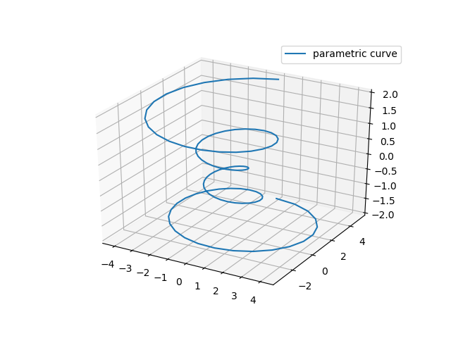
折线图
Axes3D.plot(xs,ys,*args,**kwargs)
| Argument | Description |
|---|---|
| xs, ys | x, y coordinates of vertices |
| zs | z value(s), either one for all points or one for each point. |
| zdir | Which direction to use as z (‘x', ‘y' or ‘z') when plotting a 2D set. |
import matplotlib as mpl
from mpl_toolkits.mplot3d import Axes3D
import numpy as np
import matplotlib.pyplot as plt

mpl.rcParams['legend.fontsize'] = 10

fig = plt.figure()
ax = fig.gca(projection='3d')
theta = np.linspace(-4 * np.pi, 4 * np.pi, 100)
z = np.linspace(-2, 2, 100)
r = z ** 2 + 1
x = r * np.sin(theta)
y = r * np.cos(theta)
ax.plot(x, y, z, label='parametric curve')
ax.legend()

plt.show()
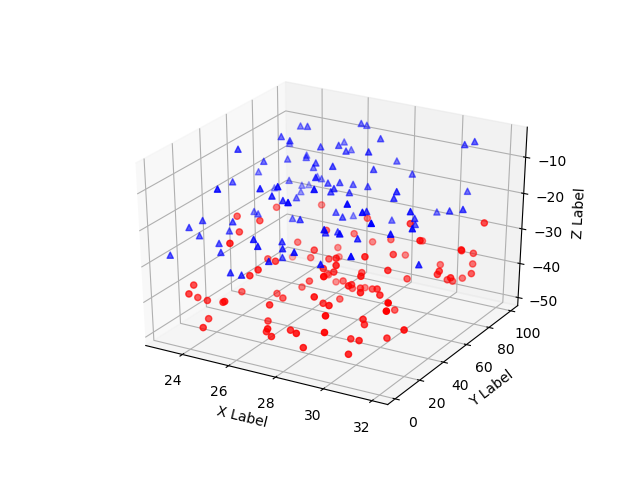
散点图
Axes3D.scatter(xs,ys,zs=0,zdir='z',s=20,c=None,depthshade=True,*args,**kwargs)
| Argument | Description |
|---|---|
| xs, ys | Positions of data points. |
| zs | Either an array of the same length as xs and ys or a single value to place all points in the same plane. Default is 0. |
| zdir | Which direction to use as z (‘x', ‘y' or ‘z') when plotting a 2D set. |
| s | Size in points^2. It is a scalar or an array of the same length as x and y. |
| c | A color. c can be a single color format string, or a sequence of color specifications of length N, or a sequence of N numbers to be mapped to colors using the cmap and norm specified via kwargs (see below). Note that c should not be a single numeric RGB or RGBA sequence because that is indistinguishable from an array of values to be colormapped. c can be a 2-D array in which the rows are RGB or RGBA, however, including the case of a single row to specify the same color for all points. |
| depthshade | Whether or not to shade the scatter markers to give the appearance of depth. Default is True. |
from mpl_toolkits.mplot3d import Axes3D
import matplotlib.pyplot as plt
import numpy as np


def randrange(n, vmin, vmax):
  '''
  Helper function to make an array of random numbers having shape (n, )
  with each number distributed Uniform(vmin, vmax).
  '''
  return (vmax - vmin) * np.random.rand(n) + vmin


fig = plt.figure()
ax = fig.add_subplot(111, projection='3d')

n = 100

# For each set of style and range settings, plot n random points in the box
# defined by x in [23, 32], y in [0, 100], z in [zlow, zhigh].
for c, m, zlow, zhigh in [('r', 'o', -50, -25), ('b', '^', -30, -5)]:
  xs = randrange(n, 23, 32)
  ys = randrange(n, 0, 100)
  zs = randrange(n, zlow, zhigh)
  ax.scatter(xs, ys, zs, c=c, marker=m)

ax.set_xlabel('X Label')
ax.set_ylabel('Y Label')
ax.set_zlabel('Z Label')

plt.show()
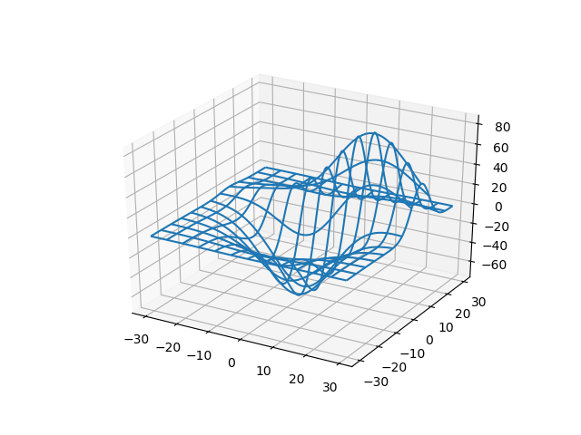
线框图
Axes3D.plot_wireframe(X,Y,Z,*args,**kwargs)
| Argument | Description |
|---|---|
| X, Y, | Data values as 2D arrays |
| Z | |
| rstride | Array row stride (step size), defaults to 1 |
| cstride | Array column stride (step size), defaults to 1 |
| rcount | Use at most this many rows, defaults to 50 |
| ccount | Use at most this many columns, defaults to 50 |
from mpl_toolkits.mplot3d import axes3d
import matplotlib.pyplot as plt

fig = plt.figure()
ax = fig.add_subplot(111, projection='3d')

# Grab some test data.
X, Y, Z = axes3d.get_test_data(0.05)

# Plot a basic wireframe.
ax.plot_wireframe(X, Y, Z, rstride=10, cstride=10)

plt.show()
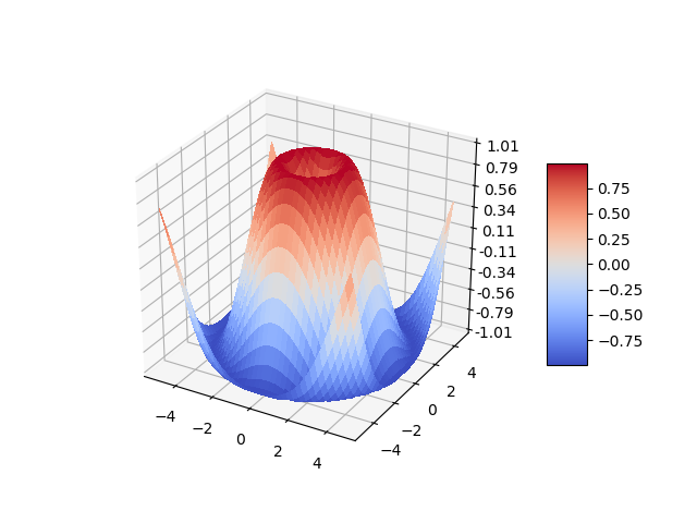
表面图
Axes3D.plot_surface(X,Y,Z,*args,**kwargs)
| Argument | Description |
|---|---|
| X, Y, Z | Data values as 2D arrays |
| rstride | Array row stride (step size) |
| cstride | Array column stride (step size) |
| rcount | Use at most this many rows, defaults to 50 |
| ccount | Use at most this many columns, defaults to 50 |
| color | Color of the surface patches |
| cmap | A colormap for the surface patches. |
| facecolors | Face colors for the individual patches |
| norm | An instance of Normalize to map values to colors |
| vmin | Minimum value to map |
| vmax | Maximum value to map |
| shade | Whether to shade the facecolors |
from mpl_toolkits.mplot3d import Axes3D
import matplotlib.pyplot as plt
from matplotlib import cm
from matplotlib.ticker import LinearLocator, FormatStrFormatter
import numpy as np

fig = plt.figure()
ax = fig.gca(projection='3d')

# Make data.
X = np.arange(-5, 5, 0.25)
Y = np.arange(-5, 5, 0.25)
X, Y = np.meshgrid(X, Y)
R = np.sqrt(X ** 2 + Y ** 2)
Z = np.sin(R)

# Plot the surface.
surf = ax.plot_surface(X, Y, Z, cmap=cm.coolwarm,
            linewidth=0, antialiased=False)

# Customize the z axis.
ax.set_zlim(-1.01, 1.01)
ax.zaxis.set_major_locator(LinearLocator(10))
ax.zaxis.set_major_formatter(FormatStrFormatter('%.02f'))

# Add a color bar which maps values to colors.
fig.colorbar(surf, shrink=0.5, aspect=5)

plt.show()
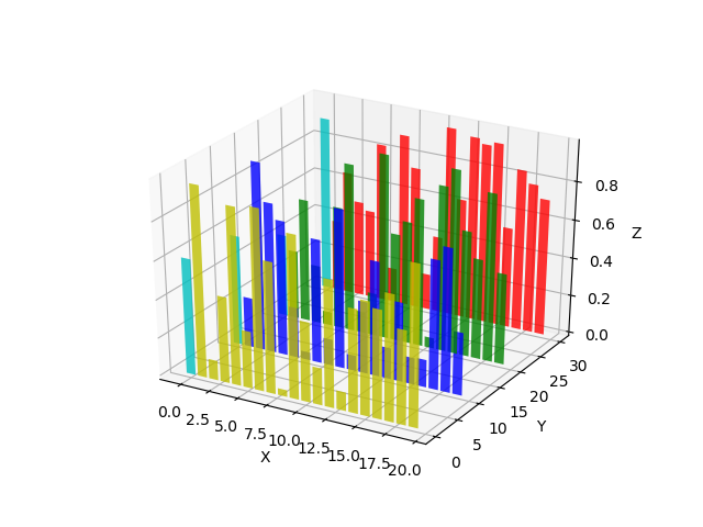
柱状图
Axes3D.bar(left,height,zs=0,zdir='z',*args,**kwargs)
| Argument | Description |
|---|---|
| left | The x coordinates of the left sides of the bars. |
| height | The height of the bars. |
| zs | Z coordinate of bars, if one value is specified they will all be placed at the same z. |
| zdir | Which direction to use as z (‘x', ‘y' or ‘z') when plotting a 2D set. |
from mpl_toolkits.mplot3d import Axes3D
import matplotlib.pyplot as plt
import numpy as np

fig = plt.figure()
ax = fig.add_subplot(111, projection='3d')
for c, z in zip(['r', 'g', 'b', 'y'], [30, 20, 10, 0]):
  xs = np.arange(20)
  ys = np.random.rand(20)

  # You can provide either a single color or an array. To demonstrate this,
  # the first bar of each set will be colored cyan.
  cs = [c] * len(xs)
  cs[0] = 'c'
  ax.bar(xs, ys, zs=z, zdir='y', color=cs, alpha=0.8)

ax.set_xlabel('X')
ax.set_ylabel('Y')
ax.set_zlabel('Z')

plt.show()
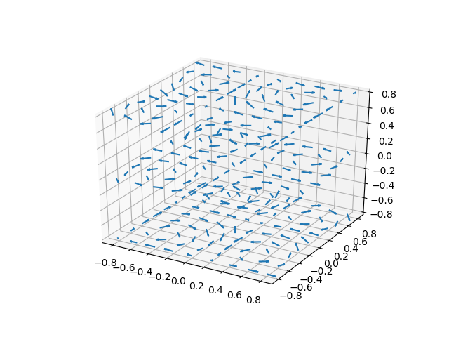
箭头图
Axes3D.quiver(*args,**kwargs)
Arguments:
X, Y, Z:
The x, y and z coordinates of the arrow locations (default is tail of arrow; see pivot kwarg)
U, V, W:
The x, y and z components of the arrow vectors
from mpl_toolkits.mplot3d import axes3d
import matplotlib.pyplot as plt
import numpy as np

fig = plt.figure()
ax = fig.gca(projection='3d')

# Make the grid
x, y, z = np.meshgrid(np.arange(-0.8, 1, 0.2),
           np.arange(-0.8, 1, 0.2),
           np.arange(-0.8, 1, 0.8))

# Make the direction data for the arrows
u = np.sin(np.pi * x) * np.cos(np.pi * y) * np.cos(np.pi * z)
v = -np.cos(np.pi * x) * np.sin(np.pi * y) * np.cos(np.pi * z)
w = (np.sqrt(2.0 / 3.0) * np.cos(np.pi * x) * np.cos(np.pi * y) *
   np.sin(np.pi * z))

ax.quiver(x, y, z, u, v, w, length=0.1, normalize=True)

plt.show()
2D转3D图
from mpl_toolkits.mplot3d import Axes3D
import numpy as np
import matplotlib.pyplot as plt

fig = plt.figure()
ax = fig.gca(projection='3d')

# Plot a sin curve using the x and y axes.
x = np.linspace(0, 1, 100)
y = np.sin(x * 2 * np.pi) / 2 + 0.5
ax.plot(x, y, zs=0, zdir='z', label='curve in (x,y)')

# Plot scatterplot data (20 2D points per colour) on the x and z axes.
colors = ('r', 'g', 'b', 'k')
x = np.random.sample(20 * len(colors))
y = np.random.sample(20 * len(colors))
labels = np.random.randint(3, size=80)

# By using zdir='y', the y value of these points is fixed to the zs value 0
# and the (x,y) points are plotted on the x and z axes.
ax.scatter(x, y, zs=0, zdir='y', c=labels, label='points in (x,z)')

# Make legend, set axes limits and labels
ax.legend()
ax.set_xlim(0, 1)
ax.set_ylim(0, 1)
ax.set_zlim(0, 1)
ax.set_xlabel('X')
ax.set_ylabel('Y')
ax.set_zlabel('Z')

# Customize the view angle so it's easier to see that the scatter points lie
# on the plane y=0
ax.view_init(elev=20., azim=-35)

plt.show()

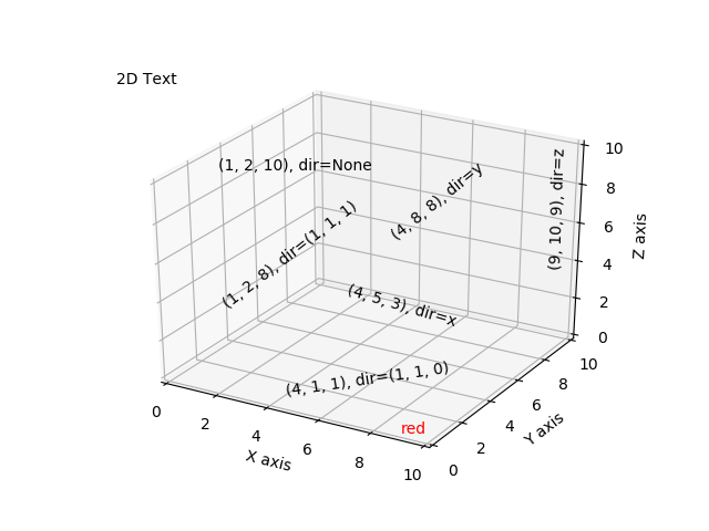
文本图
from mpl_toolkits.mplot3d import Axes3D
import matplotlib.pyplot as plt


fig = plt.figure()
ax = fig.gca(projection='3d')

# Demo 1: zdir
zdirs = (None, 'x', 'y', 'z', (1, 1, 0), (1, 1, 1))
xs = (1, 4, 4, 9, 4, 1)
ys = (2, 5, 8, 10, 1, 2)
zs = (10, 3, 8, 9, 1, 8)

for zdir, x, y, z in zip(zdirs, xs, ys, zs):
  label = '(%d, %d, %d), dir=%s' % (x, y, z, zdir)
  ax.text(x, y, z, label, zdir)

# Demo 2: color
ax.text(9, 0, 0, "red", color='red')

# Demo 3: text2D
# Placement 0, 0 would be the bottom left, 1, 1 would be the top right.
ax.text2D(0.05, 0.95, "2D Text", transform=ax.transAxes)

# Tweaking display region and labels
ax.set_xlim(0, 10)
ax.set_ylim(0, 10)
ax.set_zlim(0, 10)
ax.set_xlabel('X axis')
ax.set_ylabel('Y axis')
ax.set_zlabel('Z axis')

plt.show()
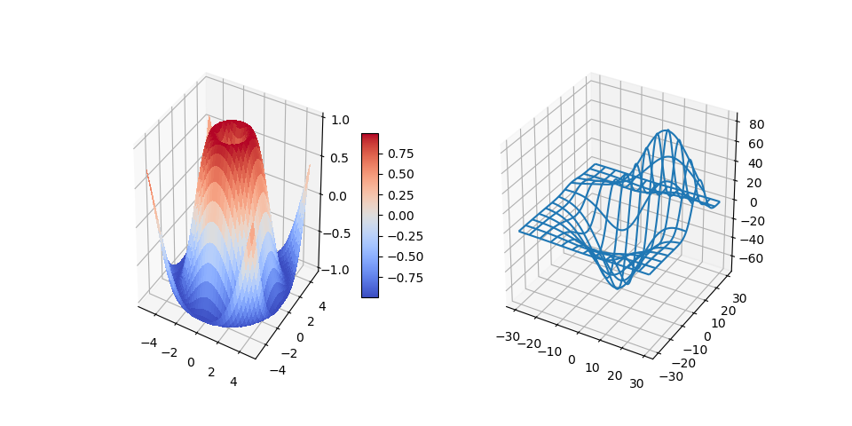
3D拼图
import matplotlib.pyplot as plt
from mpl_toolkits.mplot3d.axes3d import Axes3D, get_test_data
from matplotlib import cm
import numpy as np

# set up a figure twice as wide as it is tall
fig = plt.figure(figsize=plt.figaspect(0.5))

# ===============
# First subplot
# ===============
# set up the axes for the first plot
ax = fig.add_subplot(1, 2, 1, projection='3d')

# plot a 3D surface like in the example mplot3d/surface3d_demo
X = np.arange(-5, 5, 0.25)
Y = np.arange(-5, 5, 0.25)
X, Y = np.meshgrid(X, Y)
R = np.sqrt(X ** 2 + Y ** 2)
Z = np.sin(R)
surf = ax.plot_surface(X, Y, Z, rstride=1, cstride=1, cmap=cm.coolwarm,
            linewidth=0, antialiased=False)
ax.set_zlim(-1.01, 1.01)
fig.colorbar(surf, shrink=0.5, aspect=10)

# ===============
# Second subplot
# ===============
# set up the axes for the second plot
ax = fig.add_subplot(1, 2, 2, projection='3d')

# plot a 3D wireframe like in the example mplot3d/wire3d_demo
X, Y, Z = get_test_data(0.05)
ax.plot_wireframe(X, Y, Z, rstride=10, cstride=10)

plt.show()
到此这篇关于Matplotlib.pyplot 三维绘图的实现示例的文章就介绍到这了,更多相关Matplotlib.pyplot 三维绘图内容请搜索脚本之家以前的文章或继续浏览下面的相关文章希望大家以后多多支持脚本之家!


