
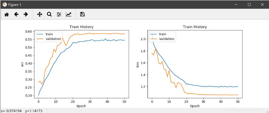
训练曲线
def show_train_history(train_history, train_metrics, validation_metrics):
 plt.plot(train_history.history[train_metrics])
 plt.plot(train_history.history[validation_metrics])
 plt.title('Train History')
 plt.ylabel(train_metrics)
 plt.xlabel('Epoch')
 plt.legend(['train', 'validation'], loc='upper left')

# 显示训练过程
def plot(history):
 plt.figure(figsize=(12, 4))
 plt.subplot(1, 2, 1)
 show_train_history(history, 'acc', 'val_acc')
 plt.subplot(1, 2, 2)
 show_train_history(history, 'loss', 'val_loss')
 plt.show()
效果:
plot(history)
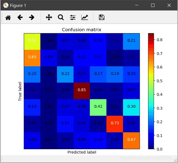
混淆矩阵
def plot_confusion_matrix(cm, classes,
    title='Confusion matrix',
    cmap=plt.cm.jet):
 cm = cm.astype('float') / cm.sum(axis=1)[:, np.newaxis]
 plt.imshow(cm, interpolation='nearest', cmap=cmap)
 plt.title(title)
 plt.colorbar()
 tick_marks = np.arange(len(classes))
 plt.xticks(tick_marks, classes, rotation=45)
 plt.yticks(tick_marks, classes)
 thresh = cm.max() / 2.
 for i, j in itertools.product(range(cm.shape[0]), range(cm.shape[1])):
 plt.text(j, i, '{:.2f}'.format(cm[i, j]), horizontalalignment="center",
   color="white" if cm[i, j] > thresh else "black")
 plt.tight_layout()
 plt.ylabel('True label')
 plt.xlabel('Predicted label')
 plt.show()

# 显示混淆矩阵
def plot_confuse(model, x_val, y_val):
 predictions = model.predict_classes(x_val)
 truelabel = y_val.argmax(axis=-1) # 将one-hot转化为label
 conf_mat = confusion_matrix(y_true=truelabel, y_pred=predictions)
 plt.figure()
 plot_confusion_matrix(conf_mat, range(np.max(truelabel)+1))
其中y_val以one-hot形式输入
效果:
x_val.shape # (25838, 48, 48, 1)
y_val.shape # (25838, 7)
plot_confuse(model, x_val, y_val)
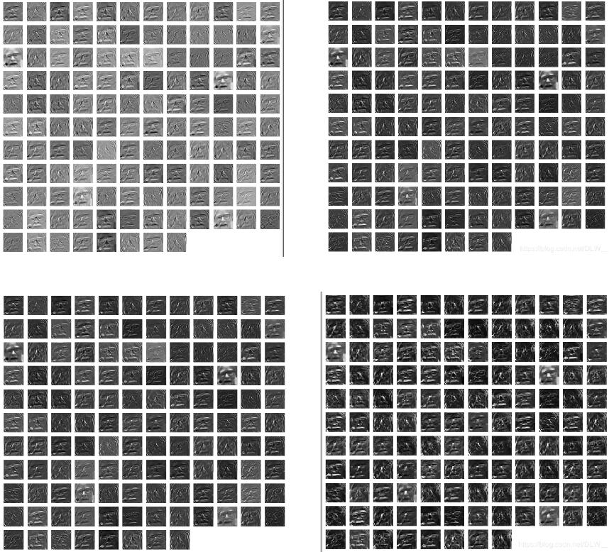
CNN层输出可视化
# 卷积网络可视化
def visual(model, data, num_layer=1):
 # data:图像array数据
 # layer:第n层的输出
 data = np.expand_dims(data, axis=0) # 开头加一维
 layer = keras.backend.function([model.layers[0].input], [model.layers[num_layer].output])
 f1 = layer([data])[0]
 num = f1.shape[-1]
 plt.figure(figsize=(8, 8))
 for i in range(num):
 plt.subplot(np.ceil(np.sqrt(num)), np.ceil(np.sqrt(num)), i+1)
 plt.imshow(f1[0, :, :, i] * 255, cmap='gray')
 plt.axis('off')
 plt.show()
num_layer : 显示第n层的输出
效果
visual(model, data, 1) # 卷积层
visual(model, data, 2) # 激活层
visual(model, data, 3) # 规范化层
visual(model, data, 4) # 池化层
补充知识:Python sklearn.cross_validation.train_test_split及混淆矩阵实现
sklearn.cross_validation.train_test_split随机划分训练集和测试集
一般形式:
train_test_split是交叉验证中常用的函数,功能是从样本中随机的按比例选取train data和testdata,形式为:
X_train,X_test, y_train, y_test =
cross_validation.train_test_split(train_data,train_target,test_size=0.4, random_state=0)
参数解释:
train_data:所要划分的样本特征集
train_target:所要划分的样本结果
test_size:样本占比,如果是整数的话就是样本的数量
random_state:是随机数的种子。
随机数种子:其实就是该组随机数的编号,在需要重复试验的时候,保证得到一组一样的随机数。比如你每次都填1,其他参数一样的情况下你得到的随机数组是一样的。但填0或不填,每次都会不一样。随机数的产生取决于种子,随机数和种子之间的关系遵从以下两个规则:种子不同,产生不同的随机数;种子相同,即使实例不同也产生相同的随机数。
示例
fromsklearn.cross_validation import train_test_split
train= loan_data.iloc[0: 55596, :]
test= loan_data.iloc[55596:, :]
# 避免过拟合,采用交叉验证,验证集占训练集20%,固定随机种子(random_state)
train_X,test_X, train_y, test_y = train_test_split(train,
             target,
             test_size = 0.2,
             random_state = 0)
train_y= train_y['label']
test_y= test_y['label']
plot_confusion_matrix.py(混淆矩阵实现实例)
print(__doc__)

import numpy as np
import matplotlib.pyplot as plt

from sklearn import svm, datasets
from sklearn.cross_validation import train_test_split
from sklearn.metrics import confusion_matrix

# import some data to play with
iris = datasets.load_iris()
X = iris.data
y = iris.target

# Split the data into a training set and a test set
X_train, X_test, y_train, y_test = train_test_split(X, y, random_state=0)

# Run classifier, using a model that is too regularized (C too low) to see
# the impact on the results
classifier = svm.SVC(kernel='linear', C=0.01)
y_pred = classifier.fit(X_train, y_train).predict(X_test)

def plot_confusion_matrix(cm, title='Confusion matrix', cmap=plt.cm.Blues):
 plt.imshow(cm, interpolation='nearest', cmap=cmap)
 plt.title(title)
 plt.colorbar()
 tick_marks = np.arange(len(iris.target_names))
 plt.xticks(tick_marks, iris.target_names, rotation=45)
 plt.yticks(tick_marks, iris.target_names)
 plt.tight_layout()
 plt.ylabel('True label')
 plt.xlabel('Predicted label')

# Compute confusion matrix
cm = confusion_matrix(y_test, y_pred)
np.set_printoptions(precision=2)
print('Confusion matrix, without normalization')
print(cm)
plt.figure()
plot_confusion_matrix(cm)

# Normalize the confusion matrix by row (i.e by the number of samples
# in each class)
cm_normalized = cm.astype('float') / cm.sum(axis=1)[:, np.newaxis]
print('Normalized confusion matrix')
print(cm_normalized)
plt.figure()
plot_confusion_matrix(cm_normalized, title='Normalized confusion matrix')

plt.show()
以上这篇keras训练曲线,混淆矩阵,CNN层输出可视化实例就是小编分享给大家的全部内容了,希望能给大家一个参考,也希望大家多多支持脚本之家。


